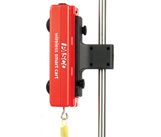
How does the PASCO Smart Cart Compare to the Vernier Go Direct® Sensor Cart?
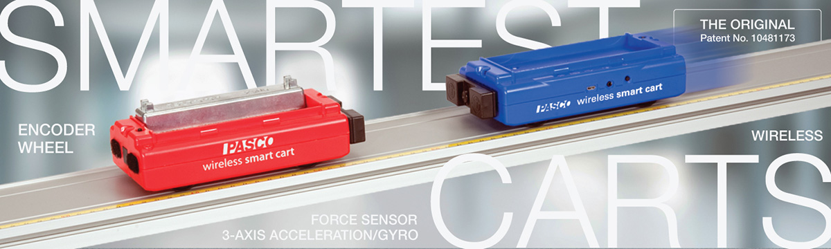
How does the PASCO Smart Cart Compare to the Vernier Go Direct® Sensor Cart?
The Smart Cart may appear to be equivalent to competitors like Vernier’s Go Direct Sensor Cart–they include many of the same features and specifications–but several distinctions set the PASCO Smart Cart apart.
What’s the Same?
Both Measure:
|
Both Feature:
|
Both Include:
|
What’s Different?
PASCO Includes More
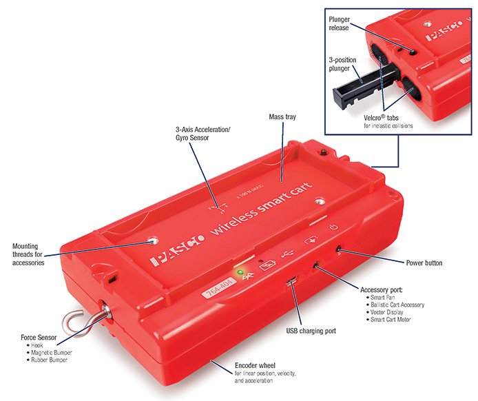
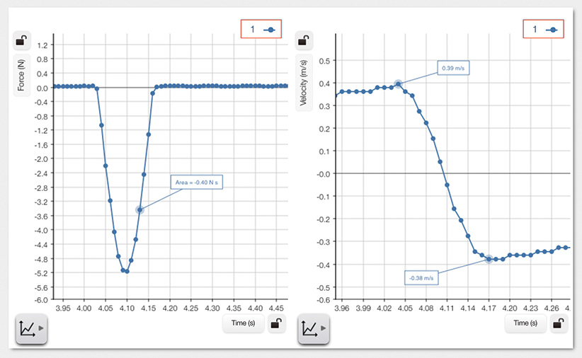
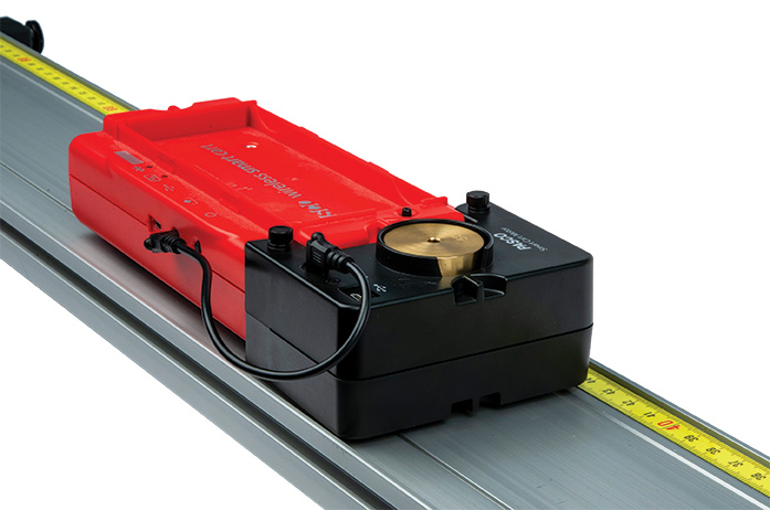
The PASCO Smart Cart comes with both hook and loop and magnetic bumpers. The magnetic bumper attaches to the force sensor, enabling you to measure the impulse during a collision. You must order bumpers separately for the Vernier sensor cart.
Why?
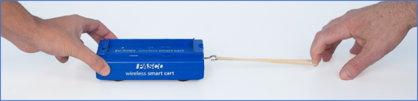
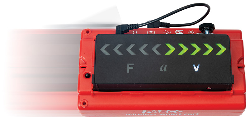
PASCO’s design makes it easy to launch the cart at 1x, 2x, and 3x velocities. With F, 2F, and 3F settings built-in to the Smart Cart, students can spend more time gathering data and solving for unknown variables and less time fiddling with cart settings.
This is important because you want to do more collisions, and with included bumpers, you can. Use the hook and loop tabs for inelastic collisions, magnetic bumper for elastic collisions, or unscrew the magnet and replace it with the rubber bumper for harder impacts.
Simple to Use Plunger
The Smart Cart plunger easily clicks into 3 different settings that correlate proportionally to 1, 2, and 3 units of force. By simply pressing the plunger to your desired setting, you can easily launch the Smart Cart at three different velocities that correlate to 1F, 2F, or 3F. Vernier’s plunger does not click into distinct velocity settings. What’s more, the total range of force on the Vernier cart is smaller than the range available to the Smart Cart, as you can only increase the force on the Vernier cart up to 1.3x.
Why?
PASCO’s design makes it easy to launch the cart at 1x, 2x, and 3x velocities. With F, 2F, and 3F settings built-in to the Smart Cart, students can spend more time gathering data and solving for unknown variables and less time fiddling with cart settings.
Larger Load Cell Capacity
PASCO’s Smart Cart load cell capacity is ±100N, double that of Vernier’s cart which is ±50N.
Why?
A larger load cell capacity means students are less likely to damage the sensor. Measure larger impulses and create collisions with higher impact. Since the sensor can withstand 100N, it is less likely to break during a tug-of-war demonstration of Newton’s 3rd Law.
Sealed & Protected Encoder Wheel
PASCO’s encoder wheel is internal and connects to the axle of an existing wheel. Vernier’s encoder wheel is an exposed 5th wheel on the underside of their Sensor Cart.
Why?
A built-in optical encoder wheel means it is sealed and protected from everyday student use. It won’t fall victim to dust, grime, or student abuse, ensuring your data is as accurate as possible for kinematics studies.
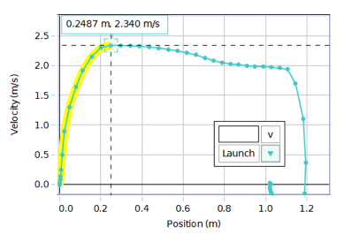
Higher Encoder Sampling Rate
PASCO’s Smart Cart encoder maximum sampling rate is 500Hz. Vernier’s rate is 30Hz.
Why?
A higher sampling rate means you can collect more data points! This is important to match a higher sampling rate of the force sensor during impulse experiments.
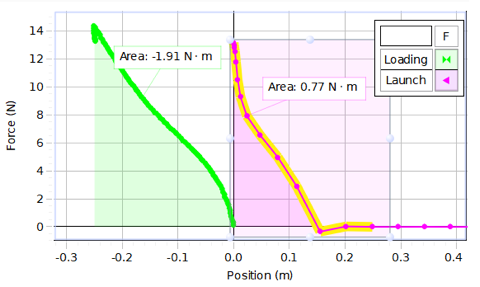
PASCO Doesn’t Manipulate the Data!
Vernier’s software performs data smoothing automatically so it cannot be turned off completely.
Why?
You’re a science educator who wants your students to collect and graph the real data, so that’s what we give you.
3-Axis Gyro
PASCO’s 3-axis accelerometer includes a 3-axis gyro, and Vernier’s 3-axis accelerometer does not.
Why?
The gyro allows you to measure angular velocity right out of the box so you can study centripetal force.
No Bumper Assembly Required
No classroom management or assembly is required to ensure the magnetic bumper is the correct orientation (north and south poles) for the Smart Cart. For the Vernier cart, you must assemble all magnetic and velcro bumpers separately, and make sure the four pieces for each Vernier cart are accounted for.
Why?
Fewer pieces and minimal assembly means easier setup, easier cleanup, and less items to lose–giving you more time for investigations.
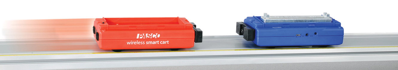
Bluetooth Time Sync Within & Between Carts
We’ve engineered our Smart Carts to time-synchronize all on-board sensors; In other words, force data syncs with velocity data from the encoder. Further, data also syncs between multiple carts in a collision so the data from both carts lines up. Vernier’s data is out of sync, and synchronization worsens as sampling rate increases.
Why?
Dependable time sync between carts means your data and graphs correlate with the phenomenon, making it easy for your students to interpret what their data is showing.
Proportional Smart Cart Masses
The Smart Cart and masses are proportional and stackable; the Smart Cart is 250 grams and the cart masses are each 250 grams. Vernier’s cart is 286 grams and the masses are 125 grams which creates strange multiples of total mass as you add masses.
Why?
Stackable and proportional masses create conceptual demonstrations and easier numbers to work into equations, aiding students in understanding core concepts.
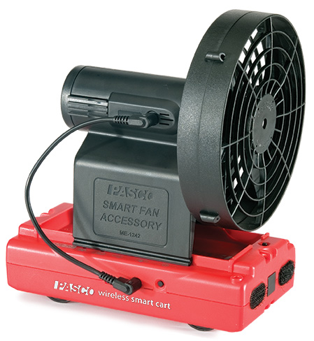
More Accessories Available
PASCO has several add-ons that pair seamlessly with our Smart Cart’s design, including a Smart Fan, Smart Ballistic Accessory, Rod Clamp, Vector Display, and Motor. Vernier does not offer any of these accessories.
Why?
Do more physics! PASCO’s accessories are designed to easily attach to the Smart Cart so students can examine core physics concepts. Also, when you connect a Smart Accessory to the Smart Cart, the Smart Cart can control the accessory for customizable investigations!
With an unparalleled design and countless applications in the physics lab, the PASCO Smart Cart will undoubtedly become one of your favorite teaching tools!
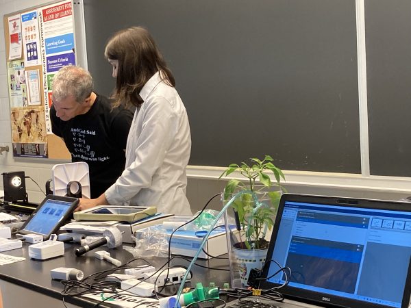 It was great to be back in person interacting with teachers! We discussed ways to integrate PASCO products into the classroom to create a fun, educational, and hands-on environment for students.
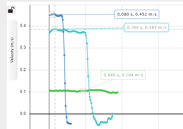 Extension: Vector Display
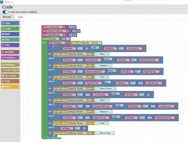 the ones I recorded, as shown in the image on the left. I tested my code by clicking start and moving the Smart Cart. At first, I was not sure where to look for the displayed text. I realized I had to change my display from a graph to digits. Then, by clicking the variable being displayed, I switched from Sensors to User-entered and chose Velocity Vector (the variable I created in the Blockly code). This time when I pressed start, the vectors I assigned to each velocity displayed on the screen depending on the Smart Cart’s speed. I decided to change the text displayed from vectors to words. As shown in the video below, I used simple terms such as slow, medium, and fast to describe the carts’ velocities.