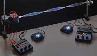
Your students will be amazed at how the PASCO strobe light instantly and dramatically freezes the motion of a vibrating string – appearing as if it’s stopped in time.
By slightly adjusting the strobe’s frequency, the string’s frozen wave will appear as if it is moving slowly forwards or backwards. This wave freezing demonstration approaches absolute zero on the ‘cool’ factor scale!
It was the shot heard across Canada. There were a lot of factors that made Kawhi’s buzzer beating basket so remarkable. Aside from there being no time left on the clock and the weight of a sport’s nation on his shoulders, Kawhi had to overcome the backward momentum that is inherent in a ‘fadeaway’. The purpose of a fadeway is to create space between the shooter and defender(s), which was a necessity for Kawhi as there were several seriously tall 76ers trying to screen his shot.
Over-coming the fadeway’s backwards momentum is no easy feat as it requires players to quickly calibrate in their minds the additional force that is required to successfully sink a basket, which for most mere mortals is not intuitive. The shot is so challenging that only a handful of NBA basketball players have been able to reliably make this shot; and we’re talking the great players such as Michael Jordan, Lebron James, Kobe Bryant and of course Kawhi Leonard.
The video below provides an extreme example of backwards momentum with a soccer ball shot from the back of a truck
Investigating Kawhi Leonard’s shot in the lab
In addition to backwards momentum there were many additional physical factors at play such as the angle of the shot and gravity. Investigating all these forces in a single activity would not be practical. Fortunately most of these forces can be isolated and explored in the lab using PASCO sensors, software and/or equipment.
Exploring The fadeaway’s negative momentum using PASCO
PASCO offers an intriguing and affordable solution to model the dramatic effect of a fadeaway’s negative momentum on projectile distance. PASCO’s mini launcher will consistently launch projectile balls the same horizontal distance for a set angle, assuming that the launcher is stationary. If however, the launcher is placed on PASCO’s frictionless cart, the force of pulling the trigger will cause the cart to move backwards at a velocity that can be measured using the motion sensor. Students will be surprised to see that even though the cart travels just a few centimeters, the overall projectile distance is significantly reduced. This can be a very simple demonstration or an in-depth quantitative analysis that factors in the projectiles initial angle and velocity, the time of flight and even the k-constant of the spring.
Other Forces Affecting a Basketball Shot
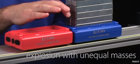
Momentum and Explosions
When a basketball player takes a jump shot (as with a fadeway), the player and the ball could be viewed as 2-object linear system if you ignore other outside forces such as gravity. What’s interesting, and perhaps not apparent to many students, is that the basketball will exert an equivalent force to the player as the player is exerting on the basketball (Newton’s 3rd Law). Of course because of the very significant inertia (mass) difference between the two objects, the basketball will accelerate at a much fast rate than the player. The player however will experience some acceleration in the opposite direction to that of the basketball.
Using Smart Carts to explore Momentum and Explosions (Free Lab)
The Wireless Smart Carts are equipped with an exploding plunger. Multiple 250g bars can be added to one cart to skew the masses. The velocities of both carts are measured using the cart’s internal position sensors enabling students to determine that momentum is conserved in a linear exploding system.
The player’s force on the basketball will be equal to the opposing force of the basketball onto the player. Of course most students will consider this a ridiculous proposition until they prove this for themselves.
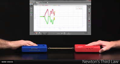
Using Smart Carts to explore Newton’s Third Law
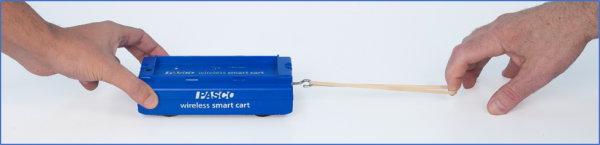
There are several ways the carts can be used. The simplest activity is for two students to have a tug-of-war using the internal force sensors of two Smart Carts and an elastic band as depicted in the image. The equal but opposite forces will be confirmed, however in relation to a basketball player taking a shot, it has some shortcomings as the forces are pulling as oppose to pushing.
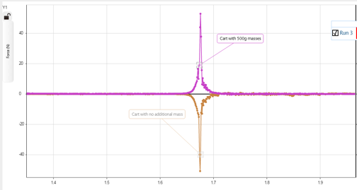
An equally simple activity, and one more relevant to the basketball shot scenario, is to collide two Smart Carts (with magnetic bumpers attached to their force sensors). As both carts have equivalent masses, students may not be surprised to see the impact forces are identical. However, what will probably surprise your students, are the force measurements that occur during a collision when one cart is weighed down with one or more 250g masses. Using their intuition, most students will speculate that one of the carts will experience a much greater force than the other. Of course, Newton’s 3rd Law will triumph and the forces will be identical.
Gravity
What goes up must come down. This is true of course for all earth bound objects (including basketballs) due to the ever present force of gravity. Without gravity the trajectory of a basketball player’s shot would be straight to the ceiling of the arena, where most of the fans would be viewing the game.
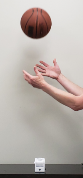
Exploring the accelerating force of gravity using the Motion sensor
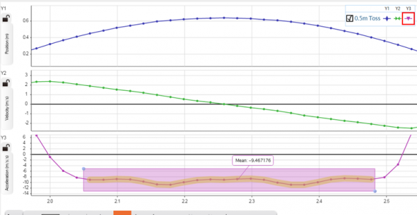
PASCO offers several technologies and techniques for measuring gravity including the Wireless Smart Gate and Picket Fence and the new Freefall apparatus. Both of these techniques are accurate and precise means to measure gravity. A third technique and one more appropriate for relating to a basketball shot is to measure the position of a vertically tossed ball and then have the software derive an acceleration graph from this data. Statistics, including the Mean of the acceleration plot can be calculated by the software for the period when the ball was in freefall as shown in the graph.
The average acceleration in the free fall period is approximately -9.5 m/s/s
Turn it on and open your choice of software: SPARKvue or Capstone.
Wirelessly connect to the Smart Cart.
Change the sample rate of the Smart Cart Position and Force sensors to 40 Hz.
Make a graph of Force vs. Position and another graph of Velocity vs. Time.
Install the hook on the Smart Cart’s force sensor. Without anything touching the force sensor, zero the force sensor in the software.
Put a rubber band on the force sensor hook. Start recording and while one person holds the rubber band in place, the other person slowly pulls the cart back, stretching the rubber band. Then hold the cart in place with the rubber band stretched and stop recording. Do not let go of the cart or rubber band.
Start recording again. Let go of the cart and move the hand holding the rubber band out of the way. Let the cart go up to its maximum speed and then stop recording.
Analysis
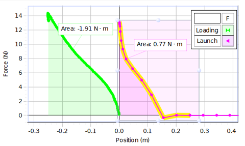
Determine the work done in stretching the rubber band by finding the area under the Force vs. Position curve.
Determine the work done as the stretched rubber band pulls the cart by finding the area under the Force vs. Position curve.
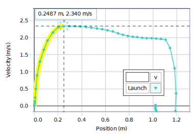
On the Velocity vs. Time graph, determine the maximum velocity. Calculate the kinetic energy of the cart and compare to the work done to accelerate the cart.
Why isn’t the work done to stretch the rubber band equal to the work done to accelerate the cart?
Sample Data
The work done loading the rubber band is -1.91 Nm. The work done unloading (when the cart is launched) the rubber band is 0.77 Nm. The resulting kinetic energy of the cart is
KE = ½ mv2 = ½ (0.252 kg)(2.34 m/s)2 = 0.69 J. This is 10% less than the energy available in the stretched rubber band.
The energy stored in the rubber band is less than the work done to stretch the rubber band. Some of that energy goes into heating the rubber band and making the rubber band move.
Turn it on and open your choice of software: SPARKvue or Capstone.
Wirelessly connect to the Smart Cart.
Make a graph of Force vs. Position.
Make sure the Smart Cart Force sensor (with the magnetic bumper on it) is not touching anything and then zero the Force sensor in the software.
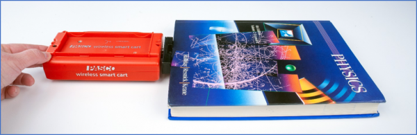
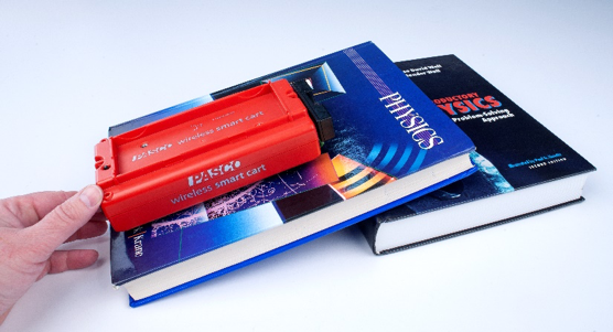
Set the cart bumper against the book. Start recording. Very slowly push the cart until the book breaks loose and then push it steadily across the table. Stop recording.
Take another run, pushing it at a faster speed once it breaks loose.
Add a second book on top of the first book and repeat.
Analysis
For each run, record the maximum force before the book moved. This is an indication of the static friction. If you can find the mass of the book, you can calculate the static coefficient of friction for the book on the table.
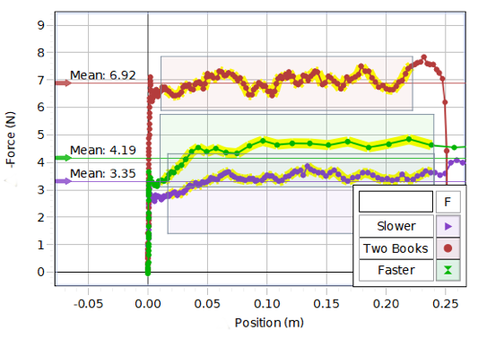
For each run, record the average force while the book was moving. This is an indication of the kinetic friction. If you can find the mass of the book, you can calculate the kinetic coefficient of friction for the book on the table.
What effect does speed have on the kinetic friction?
What changes when the extra book is added? Do the coefficients of static and kinetic friction change?
Sample Data
The average kinetic friction for two books is 6.92 N.
The average kinetic friction for one book going slower vs. faster was 3.35 N compared to 4.19 N. This indicates that the speed does influence the kinetic friction slightly.
Hooke’s Law states:
where F is the force of the spring, k is the spring constant, and x is the distance the spring has been stretched.
Take your Smart Cart out of the box.
Turn it on and open your choice of software: SPARKvue or Capstone.
Wirelessly connect to the Smart Cart.
Make a graph of Force vs. Position.
Install the hook on the Smart Cart Force Sensor. Make sure the Smart Cart Force sensor is not touching anything and then zero the Force sensor in the software.
Put one end of a spring on the hook and hold the other end stationary with your hand. Move the cart slightly to put a little tension on the spring.
Start recording and pull the Smart Cart away from the fixed end of the spring until the spring is stretched out. Then stop recording.
Analysis
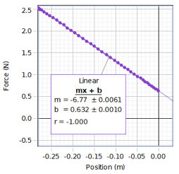
On the Force vs. Position graph, apply a linear fit to the straight-line part of the graph.
Determine the spring constant from the slope of the linear fit.
Sample Data
The slope of the graph indicates the spring constant is 6.77 N/m.
In the software, you will need to create a graph of Force vs. Acceleration.
In SPARKvue:
Under “Quick Start Experiments” choose: Impulse
Increase the sampling rate of the Force sensor to 1KHz
In Capstone:
Create two graph displays
Graph 1: [Force] vs. Time
Graph 2: [Velocity] vs. Time
Increase the sampling rate of the Force sensor to 1KHz
You will push the cart into a barrier such that the rubber bumper will collide and bounce the cart off the barrier. A wall, book or other solid vertical surface will work.
Data Collection:
Zero the force sensor
Press the record data button
With the rubber bumper facing towards the barrier, give the Smart Cart a push.
After the Smart Cart has reversed direction, stop data collection.
Data Analysis:
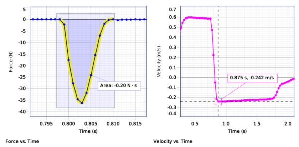
On the Force vs. Time graph, use the Area tool to measure the area under the curve. This is the impulse that the Smart Cart experienced.
On the Velocity vs. Time graph, use the Coordinate tool to find the velocity just before the impact of the Smart Cart against the barrier and record this value. This is the Smart Cart’s initial velocity.
Next, using the Coordinate tool find the velocity after the collision with the barrier. Record this value. This is the Smart Cart’s final velocity.
Weigh the cart without any bumper and record the mass. You may also estimate the mass of the Smart Cart to be around 0.250 kg.
Calculate the change in momentum of the Smart Cart: pf – pi
Compare your calculated value to the area under the Force vs. Time graph.
Sample Data:
This data was created with a Smart Cart that measured 0.246 kg, for an error around 1.5%.
Turn it on and open your choice of software: SPARKvue or Capstone.
Wirelessly connect to the Smart Cart.
Make a graph of Acceleration-x (from the Smart Cart Acceleration Sensor) vs. Angular Velocity-y (from the Smart Cart Gyro Sensor). Add a second plot area with the Force vs. Angular Velocity-y.
Install the rubber bumper on the Smart Cart Force Sensor. With the cart sitting still, with nothing touching the rubber bumper on the Force Sensor, zero the Acceleration-x, Angular Velocity-y, and the Force in the software.
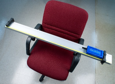
Set up a board or track on a rotatable chair as shown in the picture. Set the end stop near the end of the track and place the cart’s rubber bumper (Force Sensor end) against the end stop.
Spin the chair and start recording. Let the chair spin down to a stop and then stop recording.
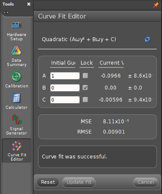
Apply a curve fit to the data to determine how the centripetal acceleration and force are related to the angular velocity. For the quadratic fit, open the curve fit editor at right in Capstone and lock the coefficient B = 0.
This forces the fit to Aω2 + C. From the curve fit, what is the radius?
In which direction are the centripetal acceleration and the centripetal force?
Further Study
Move the end stop 5 cm closer to the center of rotation. Repeat the experiment.
Continue to move the end stop closer to the center in 5 cm increments.
How does the centripetal force depend on the radius?
Sample Data
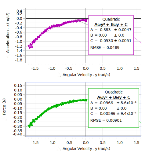
Both the centripetal acceleration and the centripetal force are pointing toward the center of the circle (they are negative) and are proportional to the square of the angular velocity.
a = -0.383ω2 – 0.0530
F = -0.0966ω2 – 0.00596
m = 0.25 kg
F = ma = 0.25(-0.383ω2 – 0.0530) = -0.096ω2 – 0.013
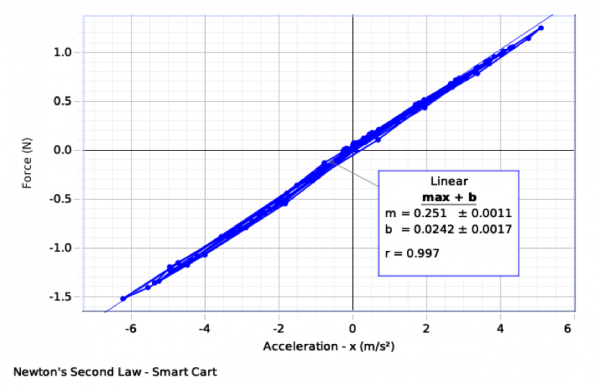
Forces and Accelerations of objects have a linear relationship that relates the mass of an object being accelerated to an unbalanced force acting on it.
Experimental Setup:
Take your Smart Cart out of the box.
Attach the hook accessory (included with Smart Cart) to the force sensor on the Smart Cart.
Press the power button on the side of the Smart Cart to turn it on.
In SPARKvue or Capstone, pair the Smart Cart to your computer or device. Here are a couple short videos to help you pair in either software:
In the software, you will need to create a graph of Force vs. Acceleration.
SPARKvue: Under “Quick Start Experiments” choose: Newton’s Second Law
Capstone:
Create a Graph Display
Select measurement of [Force] for the y-axis
Select measurement of [Acceleration – x] for the x-axis
In the sampling control panel, press the “Zero Sensor” button
Before you collect data, practice rolling the cart in a forwards and backwards motion by only holding on to the hook. You want to apply a force along the cart’s x-axis, and have the cart roll only along this direction. This is made easier using a PASCO track to keep the cart moving in one direction, but not necessary for the demonstration. (Hint: Try not to wiggle or knock the Smart Cart hook as this will result in extraneous data points.)
Data Collection:
Press the record data button
Holding only the hook, roll the Smart Cart forwards and backwards in the x-direction.
Repeat this motion a few times to generate enough data points to see the graphical relationship.
Stop data collection
Data Analysis:
Turn on the ‘Linear Fit’ tool
This relationship shows that there is a proportionality constant between the unbalanced force, and the Smart Cart’s resulting acceleration.
The proportionality constant is the mass of the cart.
Add mass to the Smart Cart and repeat data collection for the new system mass.
Sample Data:
This data was created with a Smart Cart that measured .246 kg, for an error around 2%.
Turn it on and open your choice of software: SPARKvue or Capstone.
Wirelessly connect to the Smart Cart. Change the sample rate of the Position Sensor to 40 Hz.
Open the calculator in the software and make the following calculation:
speed=abs([Velocity, Red (m/s)]) with units of m/s
Create a graph of Velocity vs. Time and add a second plot area of speed vs. Time and add a third plot area of Position vs. Time.
Mark a starting point with a piece of tape.
Start recording. Push the cart about 20 cm out and back, ending at the same point where you started.
Analysis
On the Velocity vs. Time graph, find the maximum positive velocity.
What is the instantaneous velocity at the point where you reversed the cart?
What is the average velocity over the entire motion of the cart? Highlight the area of the Velocity vs. Time graph during the time of the motion and turn on the mean statistic.
What is the average speed over the entire motion of the cart? Highlight the area of the speed vs. Time graph during the time of the motion and turn on the mean statistic.
What is the difference between speed and velocity?
Sample Data
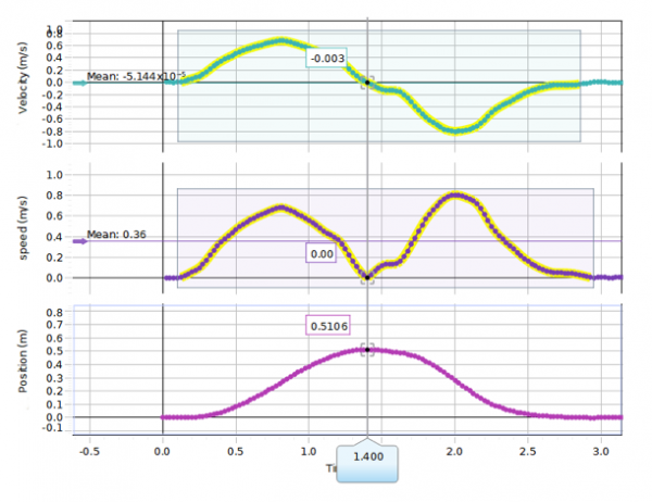
The instantaneous velocity when the cart reversed was zero.
The average velocity over the whole trip was zero because we started and stopped in the same place.
The average speed over the whole trip was 0.36 m/s.
Speed is a scalar that is the magnitude of the velocity. Velocity is a vector and has both magnitude (speed) and direction.
Turn it on and open your choice of software: SPARKvue or Capstone.
Wirelessly connect to the Smart Cart.
Change the sample rate of the Smart Cart Position sensor to 40 Hz.
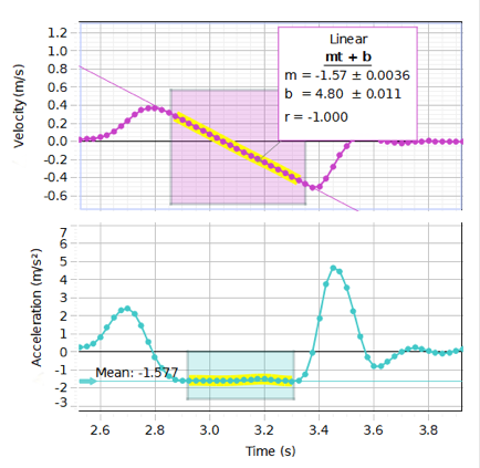
Set up a graph of Velocity vs. Time and Acceleration vs. Time using the Position sensor’s Velocity and Acceleration.
Make an inclined plane by placing the top edge of one textbook on top of a second textbook.
Put the Smart Cart at the bottom of the incline, with its force sensor end oriented up the incline.
Start recording and push the cart so it just barely reaches the top of the incline and then rolls back down. Stop recording when it gets back down.
Examine the graphs and determine where the cart is:
going up the incline.
going down the incline.
at the top of the incline.
For each of these cases, is the velocity positive, negative, zero, and/or constant? Is the acceleration positive, negative, zero, and/or constant?
When the cart is going up the incline, which direction is the velocity? Which direction is the acceleration? Is the cart accelerating or decelerating?
When the cart is at the top of the incline, the velocity is zero. Which direction is the acceleration? Is the cart accelerating or decelerating?
When the cart is going down the incline, which direction is the velocity? Which direction is the acceleration? Is the cart accelerating or decelerating?
On the Velocity vs. Time graph, find the slope of the straight-line portion. Compare this to the acceleration on the Acceleration vs. Time graph.
Sample Data
When the cart is going up the incline, the velocity is positive (up the incline) while the acceleration is constant and negative (down the incline). The cart is decelerating.
When the cart is at the top of the incline, the velocity is zero while the acceleration is constant and negative (down the incline). The cart is accelerating.
When the cart is going down the incline, the velocity is negative (down the incline) while the acceleration is constant and negative (down the incline).
The slope of the Velocity vs. Time graph is -1.57 m/s2. The average acceleration from the Acceleration vs. Time graph is -1.577 m/s2, which is 0.6% different from the slope.
Save & Share Cart
Your Shopping Cart will be saved and you'll be given a link. You, or anyone with the link, can use it to retrieve your Cart at any time.
Back
Save & Share Cart
Your Shopping Cart will be saved with Product pictures and information, and Cart Totals. Then send it to yourself, or a friend, with a link to retrieve it at any time.
Your cart email sent successfully :)
Marie Claude Dupuis
I have taught grade 9 applied science, science and technology, grade 10 applied, regular and enriched science, grade 11 chemistry and physics for 33 years at Westwood Senior High School in Hudson Québec. I discovered the PASCO equipment in 2019 and it completely changed my life. I love to discover, produce experiments and share discoveries. I am looking forward to work with your team.
Christopher Sarkonak
Having graduated with a major in Computer Science and minors in Physics and Mathematics, I began my teaching career at Killarney Collegiate Institute in Killarney, Manitoba in 2009. While teaching Physics there, I decided to invest in PASCO products and approached the Killarney Foundation with a proposal about funding the Physics lab with the SPARK Science Learning System and sensors. While there I also started a tremendously successful new course that gave students the ability to explore their interests in science and consisted of students completing one project a month, two of which were to be hands-on experiments, two of which were to be research based, and the final being up to the student.
In 2011 I moved back to Brandon, Manitoba and started working at the school I had graduated from, Crocus Plains Regional Secondary School. In 2018 I finally had the opportunity to once again teach Physics and have been working hard to build the program. Being in the vocational school for the region has led to many opportunities to collaborate with our Electronics, Design Drafting, Welding, and Photography departments on highly engaging inter-disciplinary projects. I believe very strongly in showing students what Physics can look like and build lots of demonstrations and experiments for my classes to use, including a Reuben’s tube, an electromagnetic ring launcher, and Schlieren optics setup, just to name a few that have become fan favourites among the students in our building. At the end of my first year teaching Physics at Crocus Plains I applied for CERN’s International High School Teacher Programme and became the first Canadian selected through direct entry in the 21 years of the program. This incredible opportunity gave me the opportunity to learn from scientists working on the Large Hadron Collider and from CERN’s educational outreach team at the S’Cool Lab. Following this, I returned to Canada and began working with the Perimeter Institute, becoming part of their Teacher Network.
These experiences and being part of professional development workshops with the AAPT and the Canadian Light Source (CLS) this summer has given me the opportunity to speak to many Physics educators around the world to gain new insights into how my classroom evolves. As I work to build our program, I am exploring new ideas that see students take an active role in their learning, more inter-disciplinary work with departments in our school, the development of a STEM For Girls program in our building, and organizing participation in challenges from the ESA, the Students on the Beamline program from CLS, and our local science fair.
Meaghan Boudreau
Though I graduated with a BEd qualified to teach English and Social Studies, it just wasn’t meant to be. My first job was teaching technology courses at a local high school, a far cry from the English and Social Studies job I had envisioned myself in. I was lucky enough to stay in that position for over ten years, teaching various technology courses in grades 10-12, while also obtaining a Master of Education in Technology Integration and a Master of Education in Online Instructional Media.
You will notice what is absent from my bio is any background in science. In fact, I took the minimum amount of required science courses to graduate high school. Three years ago I switched roles and currently work as a Technology Integration Leader; supporting teachers with integrating technology into their pedagogy in connection with the provincial outcomes. All of our schools have PASCO sensors at some level (mostly grades 4-12) and I made it my professional goal to not only learn how to use them, but to find ways to make them more approachable for teachers with no formal science background (like me!). Having no background or training in science has allowed me to experience a renewed love of Science, making it easier for me to support teachers in learning how to use PASCO sensors in their classrooms. I wholeheartedly believe that if more teachers could see just how easy they are to use, the more they will use them in the classroom and I’ve made it my goal to do exactly that.
I enjoy coming up with out-of-the-box ways of using the sensors, including finding curriculum connections within subjects outside of the typical science realm. I have found that hands on activities with immediate feedback, which PASCO sensors provide, help students and teachers see the benefits of technology in the classroom and will help more students foster a love of science and STEAM learning.
Michelle Brosseau
I have been teaching since 2009 at my alma mater, Ursuline College Chatham. I studied Mathematics and Physics at the University of Windsor. I will have completed my Professional Master’s of Education through Queen’s University in 2019. My early teaching years had me teaching Math, Science and Physics, which has evolved into teaching mostly Physics in recent years. Some of my favourite topics are Astronomy, Optics and Nuclear Physics. I’ve crossed off many activities from my “Physics Teacher Bucket List”, most notably bungee jumping, skydiving, and driving a tank.
Project-based learning, inquiry-based research and experiments, Understanding by Design, and Critical Thinking are the frameworks I use for planning my courses. I love being able to use PASCO’s sensors to enhance the learning of my students, and make it even more quantitative.
I live in Chatham, Ontario with my husband and two sons.
 Gravity